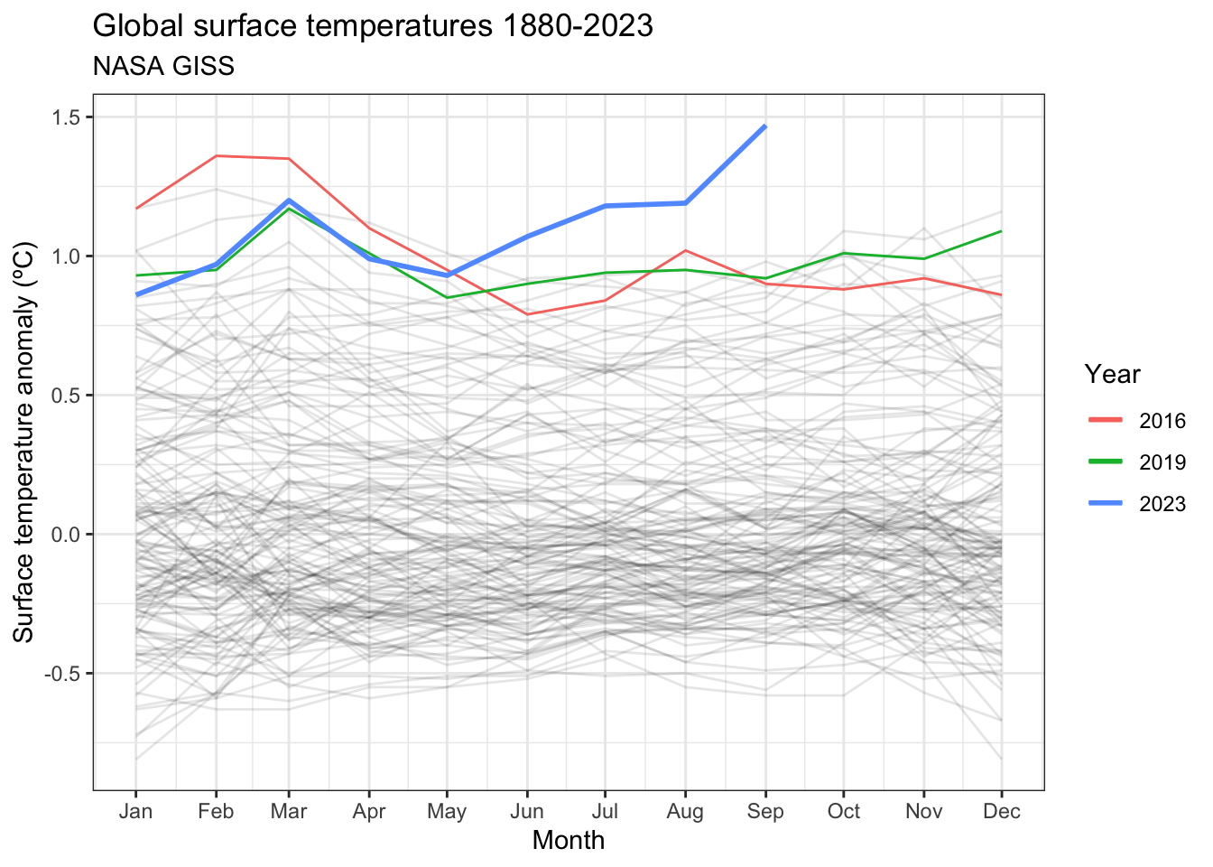
Seeing the Environmental Forest - New record for largest monthly anomaly ever

Well, it’s happened. Pending revisions to the NASA GISS record, September 2023 has gone down as the month with the largest anomaly on record. September 2023 was a jaw-dropping 1.47ºC above the 1951-1980 baseline average for September, obliterating February 2016’s 1.36ºC anomaly.

Show the code

library(tidyverse)

GISS.og <- read_table("https://data.giss.nasa.gov/gistemp/tabledata_v4/GLB.Ts+dSST.txt", 
                   skip = 7,
                   na = c("***", "****")) %>%
        filter(!row_number() %in% c(22,43, 64, 85, 106, 127, 148)) %>%
        filter(row_number() <= n() - 5)

GISS <- GISS.og %>%
        select("Year",
               "Jan",
               "Feb",
               "Mar",
               "Apr",
               "May",
               "Jun",
               "Jul",
               "Aug",
               "Sep",
               "Oct",
               "Nov",
               "Dec") %>%
        pivot_longer(!Year, 
                     names_to = "Month", 
                     values_to = "anomaly") %>%
        mutate(anomaly = as.numeric(anomaly),
               anomaly = anomaly / 100,
               Year = as.numeric(Year))

GISS$Month <- match(GISS$Month, month.abb)
GISS$Date <- make_date(year = GISS$Year, month = GISS$Month, day = 1)

GISS %>%
        mutate(Year = factor(Year),
               Date = update(Date, year = 1)) %>%
        ggplot(aes(x = Date, y = anomaly, colour = Year)) +
        scale_x_date(date_breaks = "1 month", date_labels = "%b") +
        geom_line(aes(group = Year), colour = "black", alpha = 0.1) +
        geom_line(data = function(x) filter(x, Year == 2016), lwd = 0.5) +
        geom_line(data = function(x) filter(x, Year == 2019), lwd = 0.5) +
        geom_line(data = function(x) filter(x, Year == 2023), lwd = 1) +
        theme_bw() +
        labs(title = "Global surface temperatures 1880-2023",
             subtitle = "NASA GISS",
             x = "Month",
             y = "Surface temperature anomaly (ºC)")

What’s especially striking to me, at least, is that normally the Southern Hemisphere summer (especially January and February) bring the warmest months relative to the baseline globally. The Earth is closest to the sun at that time so extra warmth makes sense. September? Nope. That’s normally one of the months that is closest to the baseline average.

We can’t entirely blame El Niño, either. First, it’s nowhere near as extreme as the 2016 or 1998 El Niños, yet. Second, global temperatures lag changes in ENSO by around 3 months. So we’re looking at June, when ENSO was in neutral territory. What we’re seeing is global warming when La Niña takes its foot off the brake. We haven’t even seen what will happen once El Niño hits the accelerator.

Show the code

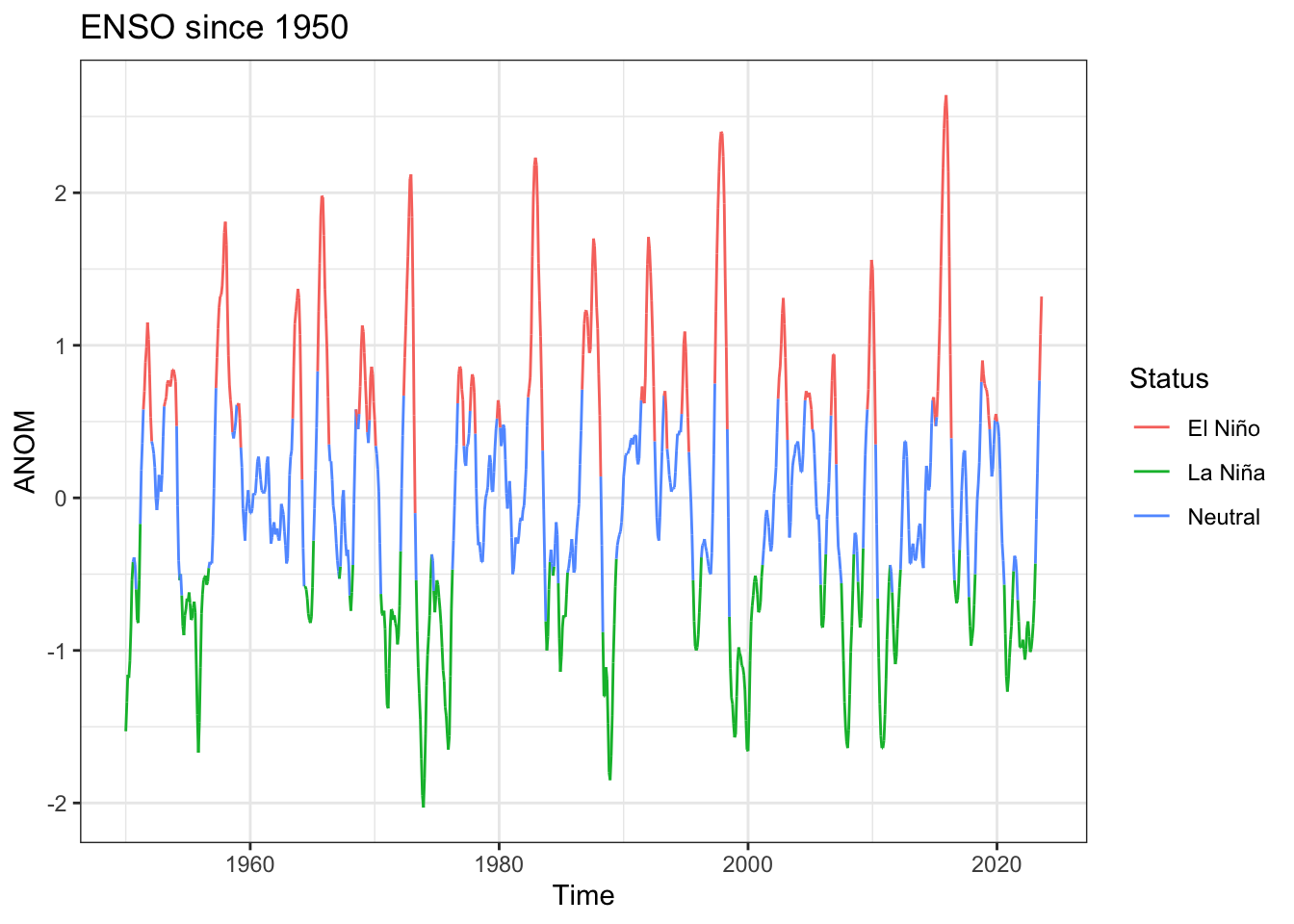
ENSO <- read_table("https://www.cpc.ncep.noaa.gov/data/indices/oni.ascii.txt")
ENSO$Time <- seq.Date(from = as.Date("1950-01-01"), by = "month", length.out = nrow(ENSO))
ENSO$Status <- with(ENSO,
                    ifelse(ANOM > 0.5, "El Niño",
                           ifelse(ANOM < -0.5, "La Niña",
                                  "Neutral"
                                  )
                           )
                    )

ENSO %>%
        ggplot(aes(x = Time, y = ANOM, colour = Status)) +
        geom_line(aes(group = 1)) +
        theme_bw() +
        labs(title = "ENSO since 1950",
             xlab = "Year",
             ylab = "Temperature anomalies (ºC)")

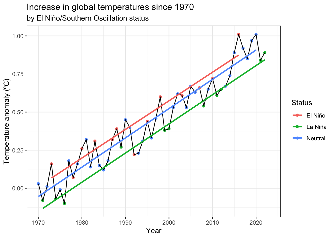
Even if the current El Niño was as extreme as 2016, we wouldn’t be able entirely blame El Niño for the recent temperature spike. Since 1970, the rate of warming is the same regardless of ENSO status. The only difference is the y-intercept baseline the trends start from.

Show the code

GISS.year <- GISS.og %>%
        select("Year",
               "J-D") %>%
        rename(anomaly = "J-D") %>%
        mutate(anomaly = as.numeric(anomaly),
               anomaly = anomaly / 100,
               Year = as.numeric(Year)) %>%
        filter(Year >= 1970) %>%
        mutate(Status = case_when(
                Year %in% c(1973, 
                            1978, 
                            1980, 
                            1983, 
                            1987, 
                            1988, 
                            1992, 
                            1995, 
                            1998, 
                            2003, 
                            2007, 
                            2010, 
                            2016) ~ "El Niño",
                Year %in% c(1971,
                            1974,
                            1976,
                            1989,
                            1999,
                            2000,
                            2008,
                            2011,
                            2012,
                            2021,
                            2022) ~ "La Niña",
                TRUE ~ "Neutral"
        ))

GISS.year %>%
        ggplot(aes(x = Year, y = anomaly)) +
        theme_bw() +
        geom_point(aes(colour = Status)) +
        geom_line(aes(group = 1)) +
        geom_smooth(aes(colour = Status), method = "lm", formula = y ~ x, se = FALSE) +
        labs(title = "Increase in global temperatures since 1970",
             subtitle = "by El Niño/Southern Oscillation status",
             x = "Year",
             y = "Temperature anomaly (ºC)")

Show the code

temp.ancova <- lm(anomaly ~ Year + Status, data = GISS.year)
summary(temp.ancova)


Call:
lm(formula = anomaly ~ Year + Status, data = GISS.year)

Residuals:
      Min        1Q    Median        3Q       Max 
-0.203246 -0.050159 -0.007132  0.058909  0.161078 

Coefficients:
                Estimate Std. Error t value Pr(>|t|)    
(Intercept)   -3.768e+01  1.421e+00 -26.525  < 2e-16 ***
Year           1.913e-02  7.127e-04  26.841  < 2e-16 ***
StatusLa Niña -1.540e-01  3.250e-02  -4.738 1.89e-05 ***
StatusNeutral -5.391e-02  2.640e-02  -2.042   0.0465 *  
---
Signif. codes:  0 '***' 0.001 '**' 0.01 '*' 0.05 '.' 0.1 ' ' 1

Residual standard error: 0.07878 on 49 degrees of freedom
  (1 observation deleted due to missingness)
Multiple R-squared:  0.9367,    Adjusted R-squared:  0.9328 
F-statistic: 241.7 on 3 and 49 DF,  p-value: < 2.2e-16

What we’re seeing this year is a normal ENSO temperature fluctuation on top of the 1.01ºC of warming we’ve experienced over the past 53 years. And it’s the warming trend, not the fluctuation, that should be getting the headlines. Without that trend, this El Niño would hardly be notable.

So yes, this El Niño will probably break global temperature records. But the only reason it’s able to do so is the overall global warming trend we’re experiencing thanks to all the CO₂ we’ve pumped into the atmosphere. And until we come to our collective senses and wean ourselves off fossil fuels, any records this El Niño sets will be temporary.

Comment Section